
CoViD-19 Data Analysis
Published by Weisser Zwerg Blog on

Some data analysis in python around the covid-19 data (including survival analysis with Kaplan-Meier).
Rationale
I’ve started to follow the development of the corona virus numbers in Europe and especially in Germany some time ago and created a few jupyter notebooks for my own use. I am in no way a medical expert and there may be mistakes in my analysis done, but I publish the notebooks on github and if you spot mistakes then please submit a pull-requests or a bug-report.
Caution
It seems that there are currently data-changes in progress that cause issues. This is mostly an issue for the US data. Once these data-changes are finalized I’ll adapt the code, but until then the US data as used in this notebook is currently wrong.
Analysis
My analysis predates the article Zahlen, bitte! 3,4 % Coronavirus-Fallsterblichkeit, eine “false Number”? Etwas Pandemie-Statistik, but the author summarizes (in german) the issues with the numbers that are floating around very well. The same reasoning that the author of that article outlines lead me to create the analysis notebooks based on raw numbers. In this blog-post I use the terminology that the author uses:
| Term | Abreviation | Definition | ||
|---|---|---|---|---|
| Confirmed Case Fatility Rate or Ratio | CFR | death / number of cases with confirmed laboratory results | ||
| Symptomatic CFR | death / estimation of symptomatic diagnosed disease cases | |||
| Infection Fatility Rate or Ratio | IFR | death / estimation of infected subjects | ||
| Crude CFR | (CFR) | Confirmed CFR estimated from the primitive: death / confirmed cases | ||
| Alternative CFR | CFRb | Confirmed CFR estimated alternatively from: death / (recovered + death) | ||
| Kaplan-Meier-CFR | CFRkm | CFR estimated via Kaplan-Meier; this estimate is taking the dynamics of the epidemic into account | ||
| Mortality Rate | death / overall population | |||
| Overall CFR or IFR | averaged over all aspects like age, sex, prior health history, … | |||
| |
||||
| A good picture representation of these numbers is given in 2019-nCoV: preliminary estimates of the confirmed-case-fatality-ratio and infection-fatality-ratio, and initial pandemic risk assessment |
The crude CFR and the alternative CFR (CFRb) are easy to estimate and you can find numbers at the bottom of covid-19-data-analysis.ipynb.
In the table the crude CFR is called death_rate and the CFRb is called death_rate_. The crude CFR is under estimating the real fatality rate,
because some of the currently infected will die. The CFRb is over-estimating the real fatality rate, because after let’s say 7 days some of the subjects died, but most of them will
recover, but are not yet counted as recovered.
For that purpose survival analysis was invented. In order to properly use survival analysis we’d need the “life-lines” of the subjects, which we don’t have. We only have aggregate numbers and we don’t know which subjects exactly died when in aggregate new death are reported. In addition we don’t know the exact date when each of the new confirmed subjects actually got infected. We only know the date when the laboratory test confirmed the infection.
For that purpose we have to artificially create the life-lines with reasonable assumptions. In case we recognize that some of our assumptions are incorrect we can modify them in the notebook to adapt as needed. You can follow the process in the covid-19-survival.ipynb notebook.
First of all I consider the data only as valid from a certain date onwards. The authorities need some time to get up-to-speed with the developing situation.
That date is called first_date. I typically use the day of the first dead person. I guess that from that day on the authorities are in full alarm state.
In case that at first_date the number of known infected persons is less than 1000 I don’t think that this number is correct (mainly to the same reasons as mentioned above,
that the authorities are not yet fully up-to-speed) and I simply add to all known confirmed cases the difference between 1000 and the number of known infected persons on that day.
This parameter is called init_add.
I also have the parameter mult available to simulate what would be the result of the analysis in case that a certain number of infected persons remain undiscovered.
This is the multiplier I multiply the confirmed cases with after adding the init_add number. In code this is:
in_df.loc[:,'confirmed'] = (in_df['confirmed'] + init_add) * multOnce this pre-processing is done I prepend the data-frame with a constant number of daily cases for 11 days. And then I prepend this data-frame again with another 11 days of
daily constant new cases. This is meant to simulate the ramp up from zero to first_date.
Based on this data I then artificially create the life-lines for the daily cases. I simply ignore the fact that subjects got infected before the day they get reported.
If it should turn out to be an important aspect of the problem then this can be changed. I use the day when subjects get reported as new_confirmed as the start date of
the life-line.
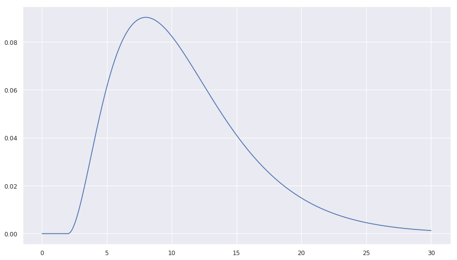
For the new_death I select the life-lines from the day before until roughly 4 weeks in the past to select randomly some life-lines that will end (simulated death). I use
a time window of 4 weeks, because I suspect that once you’re past the 4 week period you’re recovered. When selecting randomly life-lines that will end I use a
gamma distribution on the age of the life-line with parameters:
| Parameter Name | Value | |
|---|---|---|
gamma_loc |
= | 2.0 |
gamma_k |
= | 3.0 |
gamme_theta |
= | 3.0 |
| mean | = | gamma_loc + gamma_k gamme_theta = 2.0 + 9.0 |
| I use that mean, because I read somewhere that the mean (or median) of the patients time until death after hospitalization is 7 days and I guess that they are not hospitalized | ||
already on day 1. The gamma_loc of 2 days (shifts the gamme distribution right by 2 days; causes the probability of death to be 0 for that time period) also makes sure that |
||
| nobody dies in the first two days after being diagnosed. The notebook | ||
| contains a plot of the distribution (here only a static picture). |
In code this is:
    ds_age = (dt - ldf.start_date).dt.days
    distribution = stats.gamma(gamma_k, loc=2.0, scale=gamme_theta).pdf(ds_age)
    distribution = distribution / distribution.sum()

    death_indices = np.random.choice(len(ldf), new_death, replace=False, p=distribution)
If you do that then you get a CFRkm for China of 3.95%, which matches very well the 3.9% of the crude CFR. Once you have large enough numbers Kaplan-Meier does not change
the result much more.
South Korea is the other country where the situation has already a longer history. For South Korea I took as first_date 2020-02-20 and as init_add 900. I did not use a
mult parameter, because I read that South Korea is extensively testing and therefore I guess that the number of reported cases is quite close to the number of real cases.
If you do that then I get a CFRkm for South Korea of 1.16%, which is higher than the 0.7 as estimated by the crude CFR. If you would not use the init_add parameter the
CFRkm would be 1.47%.
The results in the notebook are typically reported like
(1.47, 0.97, 2.24)
(1.16, 0.86, 1.56)
8413
The first tripple belongs to the CFRkm estimate with init_add=0 and mult=1.0. The first number is the mean value estimate and the other two numbers are the lower and upper
confidence interval values.
The second tripple belongs to the CFRkm estimate with init_add and/or mult in use.
The value on the third line is the number of confirmed cases that would result with init_add and/or mult in use.
Let’s see how that works for Italy. For Italy I used first_date=2020-02-21, init_add=2000 and mult=5.0. I came up with these values by playing around with the numbers
and seeing when the resulting CFRkm seems to become “reasonable”. The results are as follows:
(27.25, 24.57, 30.16)
(3.1, 2.85, 3.38)
60745
The “raw” CFRkm without these init_add and mult adaptations would be 27.25%. As this is the same disease as in China and Korea and the fatality rate should be in the same
ballpark it is more likely that the discovery of cases is hopelessly behind the real development in Italy. If I use init_add and mult the estimate gets into the same
ballpark as for China (a bit better as I guess that the Italian health care system is a bit better than China). The consequence of this is that most likely the current number for
confirmed cases in Italy is off by a factor of 5.0! And we more likely have 61’000 cases rather than the 10’149 cases as reported by the official numbers.
For France we have a similar picture, but not as extreme as in Italy: first_date=2020-02-15, init_add=500, mult=2.0
(12.53, 8.31, 18.66)
(2.11, 1.48, 3.01)
4568
That would suggest that we have something like 4’500 cases rather than the officially reported 1’784.
Context
In 2019-nCoV: preliminary estimates of the confirmed-case-fatality-ratio and infection-fatality-ratio, and initial pandemic risk assessment the estimate of the infection-fatality-ratio (IFR) is 0.94 (0.37, 2.9) percent. The data they used can be found here.
In Coronavirus (COVID-19) Mortality Rate the reported number is 3.4%, but I cannot tell for sure if it is crude CFR or IFR or … The section How to calculate the mortality rate during an outbreak references Methods for Estimating the Case Fatality Ratio for a Novel, Emerging Infectious Disease.
The MIDAS 2019 Novel Coronavirus Repository repository on github contains more references to data and estimates.